Filters in MS Excel
Filtering data in MS Excel refers to displaying only the rows that meet certain conditions. (The other rows gets hidden.)
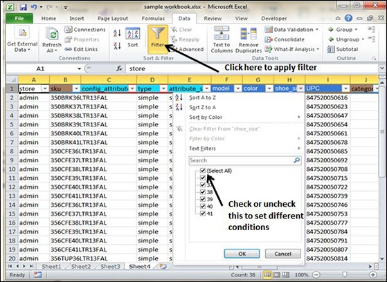
Using the store data, if you are interested in seeing data where Shoe Size is 36, then you can set filter to do this. Follow the below mentioned steps to do this.
-
Place a cursor on the Header Row.
-
Choose Data Tab » Filter to set filter.

-
Click the drop-down arrow in the Area Row Header and remove the check mark from Select All, which unselects everything.
-
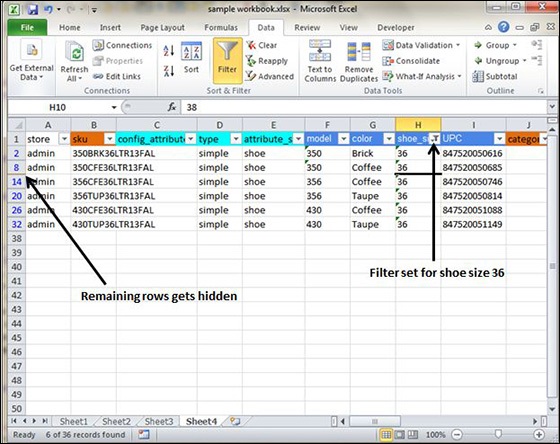
Then select the check mark for Size 36 which will filter the data and displays data of Shoe Size 36.
-
Some of the row numbers are missing; these rows contain the filtered (hidden) data.
-
There is drop-down arrow in the Area column now shows a different graphic — an icon that indicates the column is filtered.

Using Multiple Filters
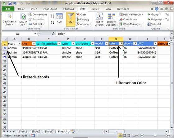
You can filter the records by multiple conditions i.e. by multiple column values. Suppose after size 36 is filtered, you need to have the filter where color is equal to Coffee. After setting filter for Shoe Size, choose Color column and then set filter for color.


